Hi!

In this new post, I will show how we can create a Data Array to extend the possibilities of the Julia package OrdinaryDiffEq.jl to simulate dynamic systems.

Necessary background

This tutorial provides additional information to solve a problem introduced by my last tutorial , then it is very important to read it before.

Problem definition

In my last post , I showed how I use the Julia package OrdinaryDiffEq.jl to simulate control systems that have continuous and discrete parts. However, there were two big problems:

1. I needed to use a global variable to pass the information from the discrete part of the system to the dynamic function (in that case, the information was the acceleration);
2. I would have to do some very bad hacks to plot the computed acceleration (creating a global vector to store the computed values).

As I mentioned, the optimal solution to circumvent those problems is was somewhat difficult to achieve. Fortunately, Chris Rackauckas , which is the maintainer of OrdinaryDiffEq.jl, introduced the concept of Data Arrays, which greatly simplified the solution for those problems. Notice that you will need v1.4.0 or higher of OrdinaryDiffEq.jl in order to have access to the new Data Array interface.

In this tutorial, the problem we want to solve is: how to create custom parameters that the discrete part of the system can modify and that will influence the dynamic function?

A little history

When I started to use OrdinaryDiffEq.jl to simulate the attitude and orbit control subsystem of Amazonia-1 satellite, I saw that I needed two kinds of variables:

1. The ones that compose the state-vector and that will be integrated by the solver; and
2. Some parameters that the control loop can modify and will influence the dynamic solution, like the commanded torque for the reaction wheels and magneto-torquers.

However, by that time, there was no easy way to achieve this. The only method was to create a custom type in Julia to store the parameters that are external to the state-vector. The problem is that you needed to implement yourself many methods in order to make this new type compatible with the OrdinaryDiffEq.jl interface. In the following, you can see what you had to do so that you can define a parameter called f1. This code was used in this issue opened by me at GitHub: https://github.com/JuliaDiffEq/DifferentialEquations.jl/issues/117

Old way to create a custom type in OrdinaryDiffEq.jl

importall Base
import RecursiveArrayTools.recursivecopy!

using DifferentialEquations

type SimType{T} <: AbstractArray{T,1}
    x::Array{T,1}

    f1::T
end

function SimType{T}(::Type{T}, length::Int64)
    return SimType{T}(zeros(length), T(0))
end

function SimType{T}(S::SimType{T})
    return SimType(T, length(S.x))
end

function SimType{T}(S::SimType{T}, dims::Dims)
    return SimType(T, prod(dims))
end

similar{T}(A::SimType{T}) = begin
    R = SimType(A)
    R.f1 = A.f1
    R
end

similar{T}(A::SimType{T}, ::Type{T}, dims::Dims) = begin
    R = SimType(A, dims)
    R.f1 = A.f1
    R
end

done(A::SimType, i::Int64) = done(A.x,i)
eachindex(A::SimType)      = eachindex(A.x)
next(A::SimType, i::Int64) = next(A.x,i)
start(A::SimType)          = start(A.x)

length(A::SimType) = length(A.x)
ndims(A::SimType)  = ndims(A.x)
size(A::SimType)   = size(A.x)

recursivecopy!(B::SimType, A::SimType) = begin
    recursivecopy!(B.x, A.x)
    B.f1 = A.f1
end

getindex( A::SimType,    i::Int...) = (A.x[i...])
setindex!(A::SimType, x, i::Int...) = (A.x[i...] = x)

Hence, Chris Rackauckas decided to create a new interface inside the OrdinaryDiffEq.jl package so that you can easily build your own custom types to be used by the solver.

Note: Actually the definition of the new interface is placed at the package DiffEqBase , which is a dependency of OrdinaryDiffEq.jl.

Data Array interface

This interface allows you to define your own types to be used by the solver. In order to do this, you just need to define a type that inherits DEDataVector:

mutable struct MyDataArray{T} <: DEDataVector{T}
    x::Vector{T}
    a::T
    b::Symbol
end

where there must be an x array that defines the state-vector and any other parameter that you will need in your simulation. Given that, you can access any of those parameters inside the solver and callback functions using u.a, u.b, etc. You can also access the i-th element of the state vector using u[i]. In other words, you do not need to use the cumbersome notation u.x[i].

This pretty much replaces all the code I showed before 👍.

Solving our problem

Hence, we now can remove the global variable a (🎉🎊🎉🎊🎉🎊) by defining the following type:

mutable struct SimWorkspace{T} <: DEDataVector{T}
    x::Vector{T}
    a::T
end

Inside our dynamic function, we can now get the commanded acceleration using u.a:

# Dynamic equation.
function dyn_eq!(du, u, t, p)
    du[1] = u[2]
    du[2] = u.a
    return nothing
end

Now, we just need to modify the affect function of our callback to write on this variable:

# Affect function.
function control_loop!(integrator)
    p = integrator.u[1]
    v = integrator.u[2]

    a = k*(r-p) + d*(0.0-v)

    for c in full_cache(integrator)
        c.a = a
    end
end

You might have noticed that there is a strange for here. This is a problem created by the internal structure of the ordinary differential equation solvers. For example, 4-th order Runge-Kutta algorithm needs to use four caches called k_1, k_2, k_3, and k_4, which are essentially the dynamic function computed at different space-state points, that are used to obtain the solution at the next sampling step. In this case, the parameter a must be set in all those caches to provide the correct solution. This is precisely what that for is doing. It is looping for all caches in the solver, and correctly setting the parametera with the acceleration computed by this callback affect function. Notice that the current state-vector integrator.u is inside the list full_cache(integrator) and, consequently, is also being set inside that loop. The good thing is that by using this for, you do not have to worry about how many caches the selected solver has.

Finally, we just need to create our initial state using the SimWorkspace type:

u0 = SimWorkspace(zeros(2), 0.0)

where the first parameter is initializing the state-vector with zeros (position and velocity), and the second parameter is initializing the acceleration. After the execution, we can access the commanded acceleration at each saved time step using sol[i].a.

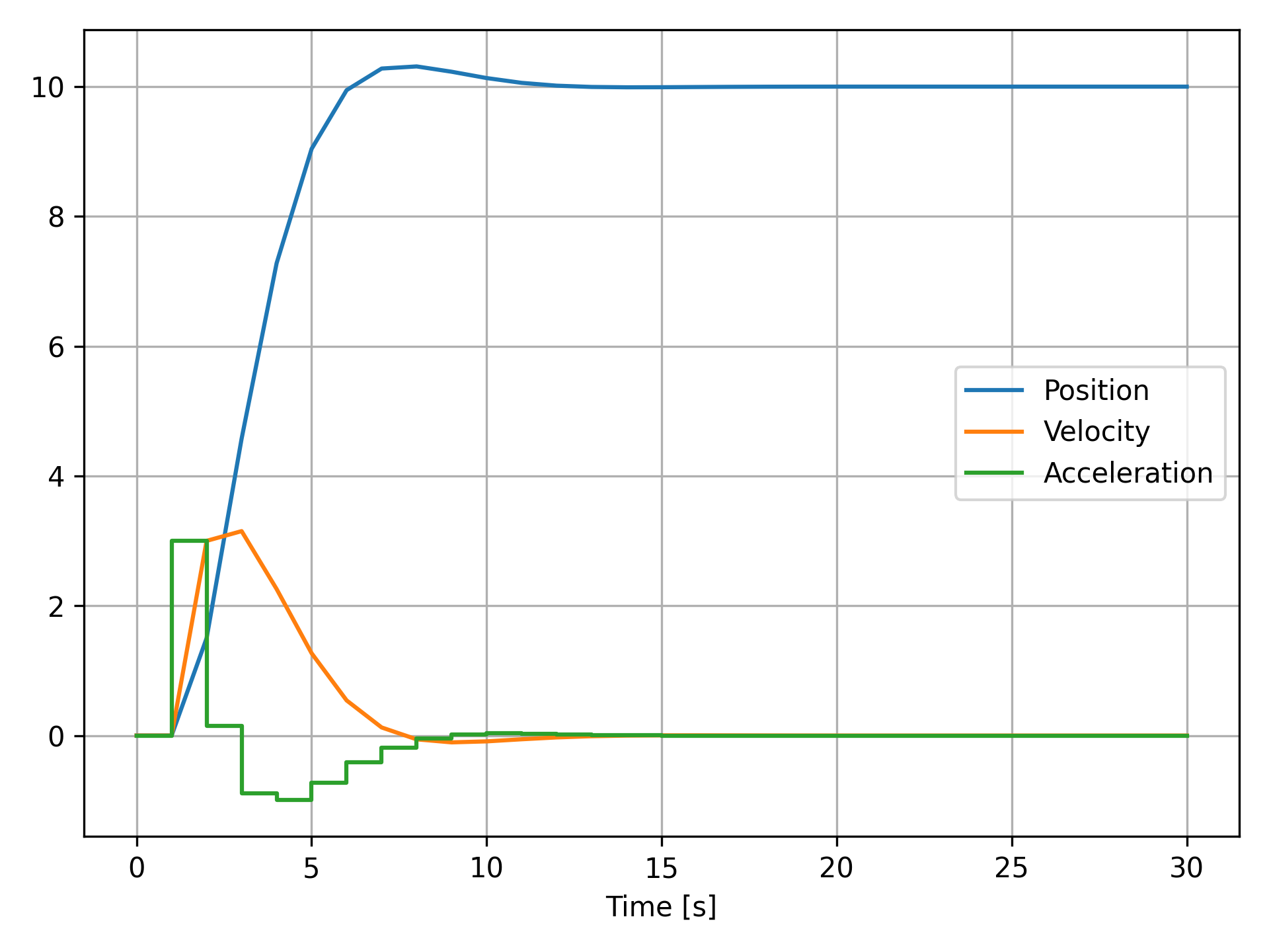
If you are using PyPlot , then the state-vector and the acceleration can be plot using:

plot(sol.t, sol.u, sol.t, map(x->x.a, sol.u))

which should provide you the following result:

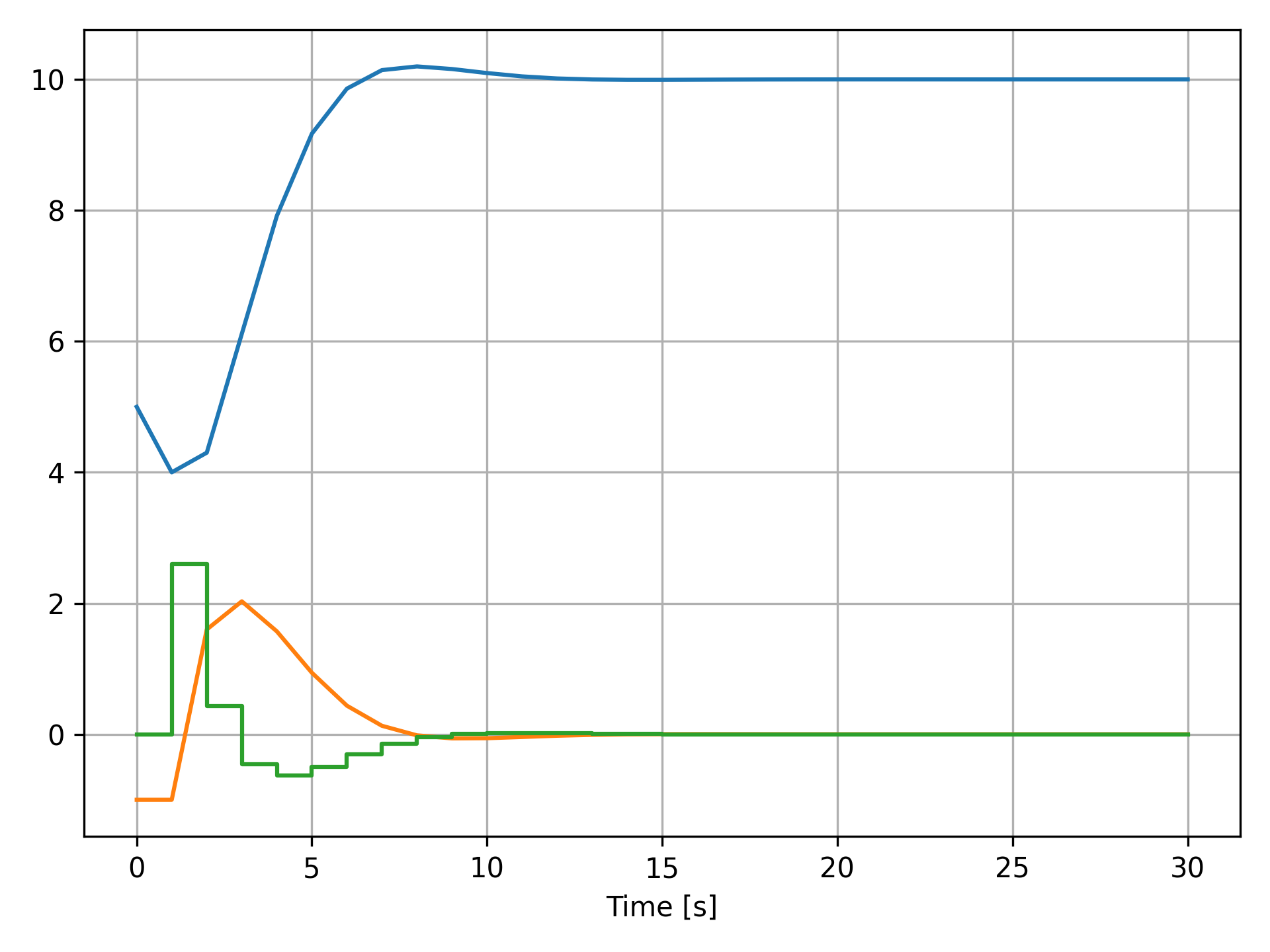
If you would like to change the initial state, then you just need to modify u0 before calling the solver:

u0 = SimWorkspace([5.0; -1.0], 0.0)

or

u0 = SimWorkspace(zeros(2), 0.0)
u0[1] = 5.0
u0[2] = -1.0

which will provide you the following result:

Conclusions

In this tutorial, I showed how you can use the Data Array interface of package OrdinaryDiffEq.jl to create your own custom simulation workspaces. Hence, now you know how to create parameters to be used inside the solver that does not belong to the state-space vector.

I provided an example by extending the solution presented in a previous tutorial , where we needed a global variable to handle this kind of parameters. Notice that, although the presented example was very simple, this concept can be easily extended to provide you an easy, elegant way to simulate much more complex systems.

If I was not very clear, please, let me know in the comments! I will use all your advice to improve this and my future tutorials!

In the following, you can find the source code of this tutorial.

using DiffEqBase
using OrdinaryDiffEq

###############################################################################
#                                 Structures
###############################################################################

mutable struct SimWorkspace{T} <: DEDataVector{T}
    x::Vector{T}
    a::T
end

###############################################################################
#                                  Variables
###############################################################################

# Parameters.
r  = 10.0   # Reference position.
k  = 0.3    # Proportional gain.
d  = 0.8    # Derivative gain.
vl = 2.0    # Velocity limit.

# Configuration of the simulation.
tf     = 30.0             # Final simulation time.
tstops = collect(0:1:tf)  # Instants that the control loop will be computed.

# Initial state of the simulation.
#                 |-- State Vector --| |-- Parameter a -- |
u0 = SimWorkspace(      zeros(2),               0.0        )

###############################################################################
#                                  Functions
###############################################################################

# Dynamic equation.
function dyn_eq(du, u, t, p)
    du[1] = u[2]
    du[2] = u.a
    return nothing
end

# CALLBACK: Control loop.
# =======================

# Condition function.
function condition_control_loop(u, t, integrator)
    (t in tstops)
end

# Affect function.
function control_loop!(integrator)
    p = integrator.u[1]
    v = integrator.u[2]

    a = k*(r-p) + d*(0.0-v)

    for c in full_cache(integrator)
        c.a = a
    end
end

cb = DiscreteCallback(condition_control_loop, control_loop!)

###############################################################################
#                                Solver
###############################################################################

prob = ODEProblem(dyn_eq, u0, (0.0, tf))
sol = solve(prob, Tsit5(), callback = cb, tstops = tstops)