The SatelliteToolbox.jl for Julia

Tutorial /Julia

2019-01-06

14 min.

Last updated: 2021-06-11

Hi!

In this tutorial, I would like to introduce the SatelliteToolbox.jl , which is a package for Julia language with many options to analyze space missions. It is used on a daily basis at the Brazilian National Institute for Space Research (INPE). First, it is presented a brief history about the package, and then I show some interesting analysis that can be done with it.

History

In 2013, I joined INPE as a Junior Space Systems Engineer. I was assigned to the space systems division in which I had to work with the attitude and orbit control subsystem (AOCS). Since I had only an intermediate knowledge about orbits, I decided to go into this subject by coding algorithms and comparing the results to the INPE heritage and to the literature in my spare time.

The very first thing was to select the language! In my Ph.D., I used MATLAB to simulate an inertial navigation system, but the Monte Carlo simulations were so slow that I had to rewrite many parts in C using CMEX. On the other hand, in my post-doctoral research where I studied estimation in distributed, non-linear systems, I decided to go with FORTRAN (using the 2008 standards to have at least a readable code…) so that the execution speed is not an issue. Yeah, the performance was very good, but it took me too much time to code. Then I heard about a new language that was promising the best of both worlds: something that resembles an interpreted language with speed of a compiled one! And that’s how I met julia .

By that time (using v0.2 I think), Julia was a really new language. But I decided to accept the rough edges and try to code my algorithms using it. Anyway, it was just a personal side project to learn more about orbits. I did face many bugs, I had to use master (pre-v0.3) due to some bugs and missing features, but it was fun 🙂

After some years (and huge rewrites due to breaking changes), Julia released its v0.4. In this time, given the amount of code I had and the state of the language, I started to see that this bunch of algorithms can indeed be used for something at INPE to help in my activities. Hence, I decided to create a private package, which was called SatToolbox.jl, to organize everything I have done.

After some time, this little side project turned out to be a very important core for a simulator, called Forplan , of the mission operational concept we started to develop at INPE’s Space Mission Integrated Design Center (CPRIME). Given the good feedback I received, I decided to rename the toolbox to SatelliteToolbox.jl and it was released as an official Julia package in March 2018 .

In this post, I would like to briefly describe SatelliteToolbox.jl and how it can be used to analyze space missions. The entire set of the features can be seen in the documentation . A brief, non-exhaustive list of the algorithms implemented by the time of this post (in v0.9.0) is:

Earth atmospheric models:
- Exponential atmospheric model;
- Jacchia-Roberts 1971;
- Jacchia-Bowman 2008 ; and
- NRLMSISE-00 .
Earth geomagnetic field models:
- IGRF v13 .
Space indices:
- Capability to automatically fetch many space indices, e.g. F10.7, Ap, Kp, etc.
Functions to perform general analysis related to orbits, e.g. converting anomalies, computing perturbations, etc.
Orbit propagators:
- Two body;
- J2;
- J4;
- Osculating J2; and
- SGP4/SDP4.
Functions to convert between ECI and ECEF references frames:
- All the IAU-76/FK5 theory is supported. Hence, the conversion between any of the following frames is available:
  - ITRF: International Terrestrial Reference Frame;
  - PEF: Pseudo-Earth Fixed reference frame;
  - MOD: Mean-Of-Date reference frame;
  - TOD: True-Of-Date reference frame;
  - GCRF: Geocentric Celestial Reference Frame;
  - J2000: J2000 reference frame;
  - TEME: True Equator, Mean Equinox reference frame.
- All the IAU-2006/2010 theory is supported. Hence, the conversion between any of the following frames is available:
  - ITRF: International Terrestrial Reference Frame;
  - TIRS: Terrestrial Intermediate Reference Frame;
  - CIRS: Celestial Intermediate Reference Frame;
  - GCRF: Geocentric Celestial Reference Frame.
Functions to convert between Geocentric and Geodetic (WGS-84) references.

In the following, I provide a few examples of how SatelliteToolbox.jl can be used to analyze space missions.

Installation

The very first thing (provided that you have Julia installed, which can be obtained here ) is to install the package. This can be done by typing:

julia> using Pkg
julia> Pkg.add("SatelliteToolbox")

If the package is already installed, then make sure you have at least the version v0.9.0. You can update all of your packages using the command Pkg.update().

To load the package, which must be done every time Julia is restarted, type:

julia> using SatelliteToolbox

Here and in the following, the command you have to type is what is presented after julia>, as you will see in the Julia REPL. Everything else is what you should see printed on the screen.

Examples

Now, I will show some analysis that can be done with the functions that are available.

Necessary background

To keep this post short, I will assume that you have knowledge about Julia and a little background in satellite and orbits.

New Year in ISS

Let’s see how can we calculate where the astronauts onboard the ISS were during the New Year in Greenwich! The first thing we need to do is to get information about the ISS orbit. In this case, we must obtain the TLE (Two-Line Element) file, which is a data format consisting of two lines with 70 characters each that contain all information related to the orbit. The following TLE was obtained from Celestrak at January 4, 2019, 12:25 +0200.

ISS (ZARYA)             
1 25544U 98067A   19004.25252738  .00000914  00000-0  21302-4 0  9994
2 25544  51.6417  96.7089 0002460 235.6509 215.6919 15.53730820149783

This TLE must be loaded into a variable inside Julia. There are a number of methods to do this using SatelliteToolbox.jl. Here, we will use a special string type:

julia> iss_tle = tle"""
       ISS (ZARYA)
       1 25544U 98067A   19004.25252738  .00000914  00000-0  21302-4 0  9994
       2 25544  51.6417  96.7089 0002460 235.6509 215.6919 15.53730820149783
       """[1]
TLE:
                     Name : ISS (ZARYA)
         Satellite number : 25544
 International designator : 98067A
       Epoch (Year / Day) : 19 /   4.25252738
       Epoch (Julian Day) : 2458487.75253 (2019-01-04T06:03:38.366)
       Element set number : 999
             Eccentricity :   0.00024600 deg
              Inclination :  51.64170000 deg
                     RAAN :  96.70890000 deg
      Argument of perigee : 235.65090000 deg
             Mean anomaly : 215.69190000 deg
          Mean motion (n) :  15.53730820 revs/day
        Revolution number : 14978
                       B* : 0.000021 1/[er]
                    ṅ / 2 : 0.000009 rev/day²
                    n̈ / 6 : 0.000000 rev/day³

This code loads the first TLE specified inside the string enclosed by tle"""...""" into the variable iss_tle.

Now, we have to initialize an orbit propagator using the loaded TLE. In this case, we will use the SGP4:

julia> orbp = init_orbit_propagator(Val(:sgp4), iss_tle)
OrbitPropagatorSGP4{Float64}(SGP4_Structure{Float64}
  epoch: Float64 2.45848775252738e6
  n_0: Float64 0.06779429624677841
  e_0: Float64 0.000246
  i_0: Float64 0.9013176963271556
  Ω_0: Float64 1.6878887209819442
  ω_0: Float64 4.112884090287905
  M_0: Float64 3.764533824882357
  bstar: Float64 2.1302e-5
  Δt: Float64 0.0
  a_k: Float64 1.0637096874073868
  e_k: Float64 0.000246
  i_k: Float64 0.9013176963271556
  Ω_k: Float64 1.6878887209819442
  ω_k: Float64 4.112884090287905
  M_k: Float64 3.764533824882357
  n_k: Float64 0.06778673761247853
  all_0: Float64 1.0637096874073868
  nll_0: Float64 0.06778673761247853
  AE: Float64 1.0
  QOMS2T: Float64 1.880276800610929e-9
  β_0: Float64 0.9999999697419996
  ξ: Float64 19.424864323113187
  η: Float64 0.005082954423839129
  sin_i_0: Float64 0.7841453225081563
  θ: Float64 0.6205772419196337
  θ²: Float64 0.3851161131885796
  A_30: Float64 2.53215306e-6
  k_2: Float64 0.000541314994525
  k_4: Float64 6.0412035375e-7
  C1: Float64 4.150340425449004e-10
  C3: Float64 0.005256030013878398
  C4: Float64 7.530189312128735e-7
  C5: Float64 0.0005696111334271365
  D2: Float64 1.4236674016273006e-17
  D3: Float64 7.305590907411524e-25
  D4: Float64 4.371134237708994e-32
  dotM: Float64 0.06779430410299993
  dotω: Float64 4.494429738092811e-5
  dotΩ1: Float64 -6.0376191376125836e-5
  dotΩ: Float64 -6.040900414071781e-5
  algorithm: Symbol sgp4
  sgp4_gc: SGP4_GravCte{Float64}
  sgp4_ds: SatelliteToolbox.SGP4.SGP4_DeepSpace{Float64}
)

The variable orbp now holds the orbit propagator structure of type SGP4 with the orbit specified by the TLE iss_tle. This TLE was generated at the Julian da 2458487.75253 (2019-01-04 06:03:38.592 +0000). Thus, we have to backpropagate the orbit to the desired instant 2019-01-01 00:00:00.000 +0000 (New Year in Greenwich). This can be accomplished by the function propagate_to_epoch! as follows:

julia> r_teme, v_teme = propagate_to_epoch!(orbp, DatetoJD(2019, 1, 1, 0, 0, 0))
([4.611518329631408e6, -976729.067497954, -4.88282144483482e6], [-998.4098394510016, 7209.562875654184, -2387.4797255179474])

The function propagate_to_epoch! returns two values. The first one r_teme is the position vector, and the second one v_teme is the velocity vector. Those vectors are represented on the same reference frame that was used to describe the orbit elements when the propagator was initialized. Since we are using the TLE, those vectors are represented in the TEME (True Equator, Mean Equinox) reference frame.

TEME is an Earth-Centered Inertial (ECI) reference frame. Hence, we must convert the position vector to an Earth-Centered, Earth-Fixed (ECEF) reference frame so that we can compute what was the ISS position (latitude, longitude, and altitude) at the desired instant. SatelliteToolbox.jl has the entire IAU-76/FK5 theory related to the conversion between reference frames . For this example, we will convert TEME into the International Terrestrial Reference Frame (ITRF) for more accurate computation. This kind of conversion requires the Earth Orientation Data (EOP) that is provided by IERS . SatelliteToolbox.jl can easily load and use this data as follows:

julia> eop = get_iers_eop()
[ Info: Downloading file 'EOP_IAU1980.TXT' from 'https://datacenter.iers.org/data/csv/finals.all.csv' with cURL.
EOPData_IAU1980:
     Data │ Timespan
 ─────────┼──────────────────────────────────────────────
        x │ 1973-01-02T00:00:00 -- 2022-06-18T00:00:00
        y │ 1973-01-02T00:00:00 -- 2022-06-18T00:00:00
  UT1-UTC │ 1973-01-02T00:00:00 -- 2022-06-18T00:00:00
      LOD │ 1973-01-02T00:00:00 -- 2021-06-09T00:00:00
       dψ │ 1973-01-02T00:00:00 -- 2021-08-24T00:00:00
       dϵ │ 1973-01-02T00:00:00 -- 2021-08-24T00:00:00

The EOP data is measured and published by IERS. This means that the ITRF cannot be used here to predict what will be the ISS position in the future since the EOP data will not be available. In this scenario, if high accuracy is not needed, then the Pseudo-Earth Fixed (PEF) reference frame can be used. The conversion between TEME and PEF using IAU-76/FK5 does not require external data.

The DCM (Direction Cosine Matrix) that rotates TEME into alignment with ITRF is computed by:

 julia> D_ITRF_TEME = rECItoECEF(TEME(), ITRF(), DatetoJD(2019,1,1,0,0,0), eop)
3×3 StaticArrays.SMatrix{3, 3, Float64, 9} with indices SOneTo(3)×SOneTo(3):
 -0.179839     0.983696     4.18981e-7
 -0.983696    -0.179839    -1.3147e-6
 -1.21792e-6  -6.48585e-7   1.0

Thus, the position vector represented in ITRF is:

julia> r_itrf = D_ITRF_TEME * r_teme
3-element StaticArrays.SVector{3, Float64} with indices SOneTo(3):
 -1.7901372297320098e6
 -4.360672082684836e6
 -4.882826427795808e6

Finally, considering the WGS-84 reference ellipsoid , the latitude, longitude, and altitude of the ISS during the New Year in Greenwich can be obtained by the function ECEFtoGeodetic as follows:

julia> lat,lon,h = ecef_to_geodetic(r_itrf)
(-0.8061562372064934, -1.9603374912499567, 419859.07333969604)

julia> rad2deg(lat)
-46.18935002007934

julia> rad2deg(lon)
-112.31906466988647

julia> h/1000
419.85907333969607

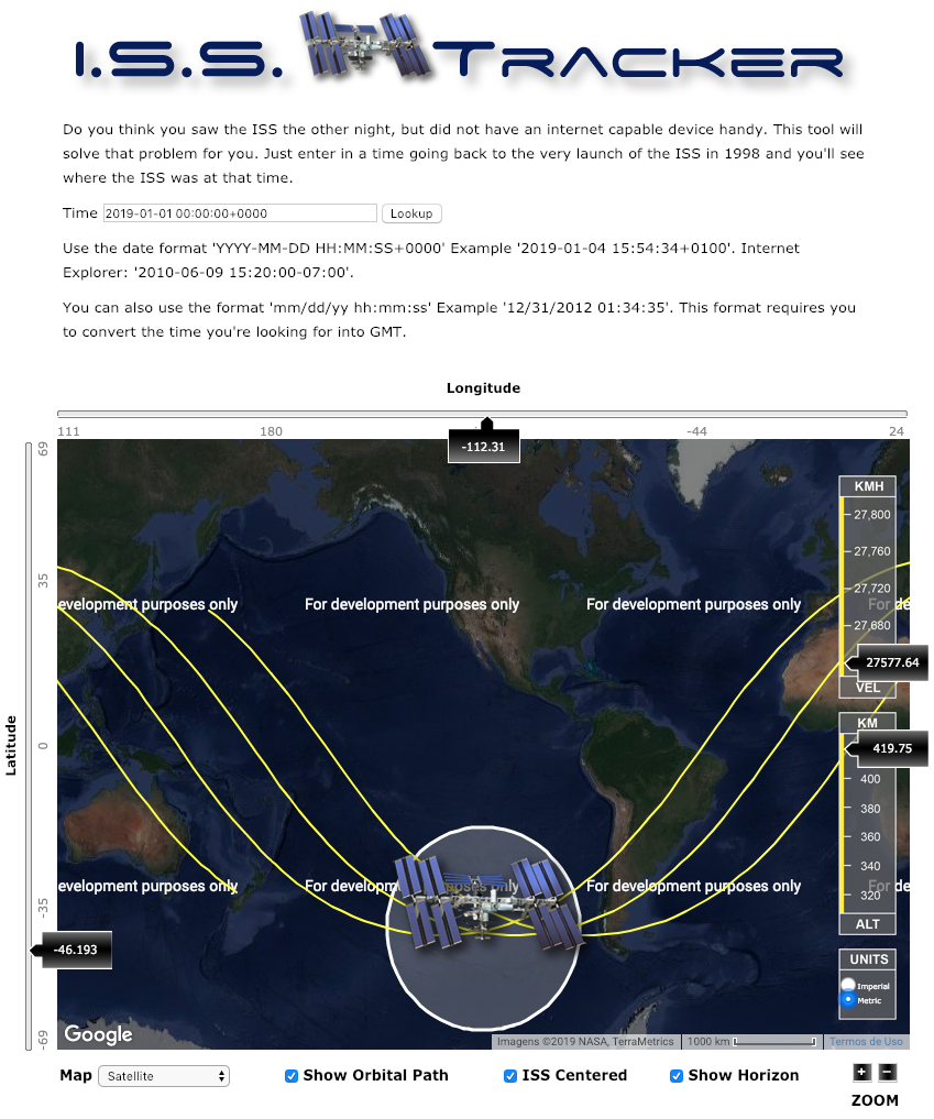
i.e., latitude 46.189° S, longitude 112.319° W, altitude 419.859 km. This is in agreement with the historical information on I.S.S. Tracker website :

The minor difference can be explained by the TLE we used to computed the ISS position and the one used by the historical data of I.S.S. Tracker. Since a TLE has errors and the propagation increases them, it is desirable to obtain a TLE as closest as possible to the desired instant, which was not pursued here.

Atmospheric density profile

In this second example, we will use the built-in functions of SatelliteToolbox.jl to compute the atmospheric density profile. There are many models available in the literature. SatelliteToolbox.jl implements four of them: Exponential atmospheric model, Jacchia-Roberts 1971, Jacchia-Bowman 2008, and NRLMSISE-00. All of them but the former requires as input some space indices, like the F10.7 that measures the Sun activity and the Ap that measures the geomagnetic activity. SatelliteToolbox.jl is prepared to download all the required files from the Internet so that those indices can be easily obtained. This can be accomplished by:

julia> init_space_indices(wdcfiles_newest_year = 2018)
[ Info: Downloading file 'DTCFILE.TXT' from 'http://sol.spacenvironment.net/jb2008/indices/DTCFILE.TXT' with cURL.
[ Info: Downloading file 'fluxtable.txt' from 'ftp://ftp.seismo.nrcan.gc.ca/spaceweather/solar_flux/daily_flux_values/fluxtable.txt' with cURL.
[ Info: Downloading file 'SOLFSMY.TXT' from 'http://sol.spacenvironment.net/jb2008/indices/SOLFSMY.TXT' with cURL.
[ Info: Downloading file 'kp2018.wdc' from 'ftp://ftp.gfz-potsdam.de/pub/home/obs/kp-ap/wdc/yearly/kp2018.wdc' with cURL.

The keyword wdcfiles_newest_year is not necessary, but it is added to avoid an error since the kp2019.wdc file was not available by the time this tutorial was written for the first time. For more information, see the documentation.

We will compute the atmospheric density profile from 100 km to 1000 km (steps of 1 km) using all the four models at 2018-11-1 00:00:00+0000 over São José dos Campos, SP, Brazil (Latitude 23.2237° S, Longitude 45.9009° W).

The exponential atmospheric model, the simpler one, depends neither on space indices nor on the location, only on the altitude. Thus, the atmospheric profile is computed by:

 julia> at_exp = expatmosphere.(100e3:1e3:1000e3)
901-element Vector{Float64}:
 5.297e-7
 4.4682006197154693e-7
 3.7690800034030025e-7
 3.1793478585921236e-7
 2.6818886298003355e-7
 2.2622647607479199e-7
 1.908297679051222e-7
 1.6097143424840973e-7
 1.357849088663833e-7
 1.1453921350666081e-7
 9.661e-8
 8.418342953216043e-8
 7.335524073901479e-8
 ⋮
 3.2081624552727763e-15
 3.190491541905968e-15
 3.1729179618829572e-15
 3.155441179080928e-15
 3.1380606603300916e-15
 3.1207758753974133e-15
 3.1035862969704423e-15
 3.086491400641224e-15
 3.069490664890299e-15
 3.0525835710707956e-15
 3.0357696033926073e-15
 3.019e-15

Each element is the atmospheric density [kg/m³] related to one altitude.

Here we use the Julia broadcast operator . to compute for the entire altitude interval using only one line. For more information, see the documentation.

For the Jacchia-Robert 2008, we must specify the geodetic latitude [rad], longitude [rad], and altitude. Notice that, since we have already initialized the space indices, all the required information will be gathered automatically:

julia> at_jb2008 = jb2008.(DatetoJD(2018, 11, 1, 0, 0, 0), deg2rad(-23.2237), deg2rad(-45.9009), 100e3:1e3:1000e3)
901-element Vector{JB2008_Output{Float64}}:
 JB2008_Output{Float64}
  nN2: Float64 8.667790698990597e18
  nO2: Float64 2.0068762518417774e18
  nO: Float64 6.369594178974921e17
  nAr: Float64 1.0364507121824598e17
  nHe: Float64 1.430390758033398e14
  nH: Float64 0.9692087748575587
  rho: Float64 5.33599234410689e-7
  T_exo: Float64 682.1900524076311
  Tz: Float64 193.07856649704962

 JB2008_Output{Float64}
  nN2: Float64 7.214648727684497e18
  nO2: Float64 1.64148948964543e18
  nO: Float64 5.880481385846831e17
  nAr: Float64 8.626913214258544e16
  nHe: Float64 1.1905879157579538e14
  nH: Float64 0.9677466330108101
  rho: Float64 4.441421316371682e-7
  T_exo: Float64 682.1900524076311
  Tz: Float64 195.73089787616576

 ⋮

 JB2008_Output{Float64}
  nN2: Float64 10.314784455727064
  nO2: Float64 0.008222186809865062
  nO: Float64 2.3738400239219222e7
  nAr: Float64 6.825921807010572e-9
  nHe: Float64 1.0598617834538963e11
  nH: Float64 2.1749553505283655e11
  rho: Float64 1.069027097007535e-15
  T_exo: Float64 682.1900524076311
  Tz: Float64 682.1462306202664

 JB2008_Output{Float64}
  nN2: Float64 9.948604163820175
  nO2: Float64 0.00788959257731523
  nO: Float64 2.325359614062785e7
  nAr: Float64 6.4829271673513334e-9
  nHe: Float64 1.0544232920443207e11
  nH: Float64 2.1721772409199527e11
  rho: Float64 1.0649348369412183e-15
  T_exo: Float64 682.1900524076311
  Tz: Float64 682.1464044429722

Each element is an instance of the structure JB2008_Output that contains the density of the atmospheric species in [kg/m³] related to one altitude.

The NRLMSISE-00 requires the same information, but in a different order. One more time, since we have already initialized the space indices, all the required information is fetched automatically:

julia> at_nrlmsise00 = nrlmsise00.(DatetoJD(2018, 11, 1, 0, 0, 0), 100e3:1e3:1000e3, deg2rad(-23.2237), deg2rad(-45.9009))
901-element Vector{NRLMSISE00_Output{Float64}}:
 NRLMSISE00_Output{Float64}
  den_N: Float64 3.225647667164221e11
  den_N2: Float64 1.1558415665482785e19
  den_O: Float64 4.649965500403523e17
  den_aO: Float64 4.631659520454273e-37
  den_O2: Float64 2.6263326718789934e18
  den_H: Float64 2.533162671436194e13
  den_He: Float64 1.2320073447340945e14
  den_Ar: Float64 1.1608097446818192e17
  den_Total: Float64 6.968049043353933e-7
  T_exo: Float64 1027.3184649
  T_alt: Float64 215.25904311781903
  flags: NRLMSISE00_Flags

 NRLMSISE00_Output{Float64}
  den_N: Float64 3.5691748620576013e11
  den_N2: Float64 1.0012594360559639e19
  den_O: Float64 4.6065649467733504e17
  den_aO: Float64 1.8947221849916306e-36
  den_O2: Float64 2.2358683099960123e18
  den_H: Float64 2.35052621777078e13
  den_He: Float64 1.1213184590500758e14
  den_Ar: Float64 9.845632305957742e16
  den_Total: Float64 6.029280387245405e-7
  T_exo: Float64 1027.3184649
  T_alt: Float64 213.7198609515809
  flags: NRLMSISE00_Flags

 ⋮

 NRLMSISE00_Output{Float64}
  den_N: Float64 5.1846924324256405e6
  den_N2: Float64 110.11884724745335
  den_O: Float64 7.740861835165262e7
  den_aO: Float64 2.049309406130631e9
  den_O2: Float64 0.0820328042018332
  den_H: Float64 1.3029978336346179e11
  den_He: Float64 8.29558653433061e10
  den_Ar: Float64 1.5144387918985786e-7
  den_Total: Float64 8.237307143679598e-16
  T_exo: Float64 724.4998315669409
  T_alt: Float64 724.4998315392361
  flags: NRLMSISE00_Flags

 NRLMSISE00_Output{Float64}
  den_N: Float64 5.097414213511122e6
  den_N2: Float64 106.44260908421272
  den_O: Float64 7.592117961201309e7
  den_aO: Float64 2.042142218337004e9
  den_O2: Float64 0.07891050457188623
  den_H: Float64 1.3014187084557657e11
  den_He: Float64 8.255445331597499e10
  den_Ar: Float64 1.442732462296107e-7
  den_Total: Float64 8.205713083292234e-16
  T_exo: Float64 724.4998315669409
  T_alt: Float64 724.4998315398782
  flags: NRLMSISE00_Flags

Each element is an instance of the structure NRLMSISE00_Output that contains the density of the atmospheric species in [kg/m³] related to one altitude.

The values computed here can be compared to the online NRLMSISE-00 model. Notice, however, that the online version by the time this tutorial was written only allows computation between 1960/02/14 and 2018/03/17.

The Jacchia-Roberts 1971 model does not support fetching the space indices automatically yet. Hence, we will need to do this manually. It requires three indices: the daily F10.7, the averaged F10.7 (81-day window, centered on input time), and the Kp geomagnetic index (with a delay of 3 hours). That information can be fetched by:

julia> F107 = get_space_index(F10(), DatetoJD(2018, 11, 1, 0, 0, 0))
65.8

julia> F107m = get_space_index(F10M(), DatetoJD(2018, 11, 1, 0, 0, 0); window = 81)
68.29135802469136

julia> kp = get_space_index(Kp(), DatetoJD(2018, 11, 1, 0, 0, 0) - 3 / 24)
0.875

Thus, the atmospheric profile computed by JR1971 is obtained by:

julia> at_jr1971 = jr1971.(DatetoJD(2018,11,1,0,0,0), deg2rad(-23.2237), deg2rad(-45.9009), 100e3:1e3:1000e3, F107, F107m, kp)
901-element Vector{JR1971_Output{Float64}}:
 JR1971_Output{Float64}
  nN2: Float64 5.7192521805880885e19
  nO2: Float64 1.0370130013611293e19
  nO: Float64 1.2248930040184422e19
  nAr: Float64 4.797323831280962e17
  nHe: Float64 3.150115795435398e15
  nH: Float64 0.0
  rho: Float64 3.4060767884871413e-6
  T_exo: Float64 657.167737713227
  Tz: Float64 191.2125970557249

 JR1971_Output{Float64}
  nN2: Float64 8.080629730659746e18
  nO2: Float64 1.6344357654348047e18
  nO: Float64 1.0616020508369499e18
  nAr: Float64 9.003667794720594e16
  nHe: Float64 7.366460213846506e13
  nH: Float64 0.0
  rho: Float64 4.96920849944813e-7
  T_exo: Float64 657.167737713227
  Tz: Float64 193.37386958205954

 ⋮

 JR1971_Output{Float64}
  nN2: Float64 4.99409517657604
  nO2: Float64 0.0029687873812458197
  nO: Float64 2.813594368996442e7
  nAr: Float64 1.4574247220377589e-9
  nHe: Float64 1.1029408240429312e11
  nH: Float64 3.638178032711139e11
  rho: Float64 1.3427841933298043e-15
  T_exo: Float64 669.4417264661666
  Tz: Float64 669.4417251116241

 JR1971_Output{Float64}
  nN2: Float64 4.812412406159161
  nO2: Float64 0.002845823469068375
  nO: Float64 2.7544317744479984e7
  nAr: Float64 1.3825250583995816e-9
  nHe: Float64 1.0969262471305795e11
  nH: Float64 3.63262212082261e11
  rho: Float64 1.3378408900651963e-15
  T_exo: Float64 669.4417264661666
  Tz: Float64 669.4417251377473

Each element is an instance of the structure JR1971_Output that contains the density of the atmospheric species in [kg/m³] related to one altitude.

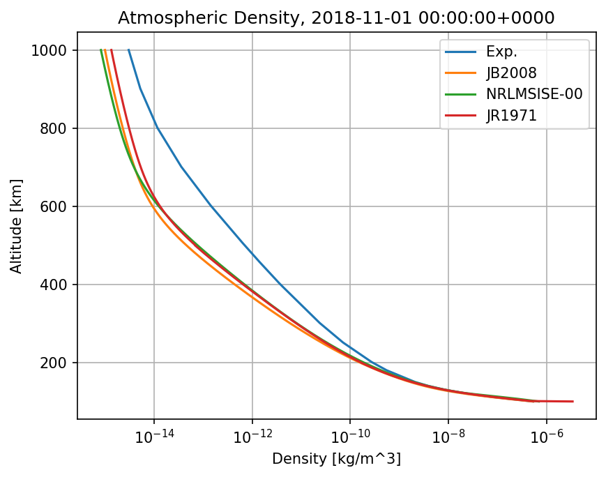
Finally, using the PyPlot.jl package, the atmospheric profiles (altitude vs. density) in semi-log scale can be plotted using:

julia> using PyPlot
julia> figure()
julia> h = 100:1:1000
julia> semilogx(at_exp, h, map(x->x.rho, at_jb2008), h, map(x->x.den_Total,at_nrlmsise00), h, map(x->x.rho,at_jr1971), h)
julia> legend(["Exp.", "JB2008", "NRLMSISE-00", "JR1971"])
julia> xlabel("Density [kg/m^3]")
julia> ylabel("Altitude [km]")
julia> title("Atmospheric Density, 2018-11-01 00:00:00+0000")
julia> grid()

which leads to:

For more information about the many options to compute the atmospheric density, please see the documentation .

If the desired date is not available on the space indices files, then an error will be thrown when computing the atmospheric density.

Conclusion

I hope that this tutorial has helped you to understand a little bit how SatelliteToolbox.jl can be used to perform analysis related to satellites and orbits. If you have any question, please, feel free to leave a comment below!

On this page

#Atmospheric models

#Julia

#Orbit

#Satellite

#SatelliteToolbox.jl