Using Julia to simulate systems composed of continuous and discrete parts

Hi!

In this first post, I would like to explain how I circumvent a problem I always had related to simulation of dynamic systems that has discrete and continuous parts. Notice that this is for sure MathWorks® Simulink territory. There is no doubt that Simulink is the faster prototyping tool for such kind of applications in which you have a continuous dynamic model modified by discrete parts that are sampled at specific time intervals.

However, sometimes there are situations in which you cannot use Simulink (not having a license being the most obvious one). In my specific use case, I am coding the Attitude and Orbit Control Subsystem (AOCS) simulator for the Amazonia-1 Satellite. Simulink gave me some problems related to simulation of some discontinuities, like shadows of some satellite parts on the coarse solar sensors. It turns out that I needed more control in the solver than Simulink could offer me. Hence, I decided to port the simulator to a “standard” language. After a very long research, Julia and the package OrdinaryDiffEq.jl provided me the best solution to simulate my system. Hence, in this post, I would like to share how I was able to solve the problem of simulating systems with discrete and continuous parts using these tools.

Necessary background

I will try to keep this tutorial as simple as possible. However, it would be helpful if you have a minimum knowledge about:

1. Julia language;
2. Control systems; and
3. Ordinary Differential Equations.

Problem definition

In most control systems, you have four parts:

1. The plant, which is what you want to control;
2. The sensors, which will measure quantities related to the processes you want to control;
3. The actuators, which will act and modify the state of your plant; and
4. The controller, which will read the sensor outputs and command the actuators to modify the plant given a set of specifications.

However, nowadays the controller is usually embedded on a microcomputer, which has predefined intervals to execute its functions. In other words, only on specific time instants (called sampling steps) the controller will read the sensor output, update the control law, and send new commands to the actuators.

In order to simulate such system, you have to consider two kinds of models: continuous and discrete. The plant, for example, is a continuous model, since it is usually modeled by a set of differential equations and generally varies for every t. The controller, as mentioned before, only updates its internal state on a determined set of time instants.

Academically speaking, the simulation of such system can be solved by using the Z-transform to convert the plant continuous model to a discrete one. Hence, every model will be discrete and can be simulated easily. This method has many problems. The biggest one, in my opinion, is that it only works for linear systems and it can be very difficult to be used in complex plants with many state variables.

Hence, the problem is: how can I use a “standard” language to simulate a system in which you have a continuous part (the plant) that is controlled by a discrete process (the controller)? I will provide in this post one possible solution using Julia and the package OrdinaryDiffEq.jl.

Proposed dynamic system

I decided to propose a very simple dynamic system to be controlled. This will help to make the tutorial more interesting and easy to understand. The problem I selected is a simple particle control in one dimension defined as follows:

This particle can be modeled by a set of two differential equations describing the time-derivative of its position and velocity:

where p is the particle position, v is the particle velocity, and a is the acceleration, which we can control.

Hence, we can define the state vector as:

Finally, our dynamic system can be written as:

Controller

We want to control the acceleration of a particle so that it goes to a specific point in space, called r. In this case, I will propose a (very) simple PD controller. The control law will be:

The controller must be a discrete process that is updated every 1s.

In the next sections, I will describe how you can use Julia and the package OrdinaryDiffEq.jl to simulate this system in a very elegant solution. You will see that you can easily extend this idea to handle much more complex systems.

Why did I choose Julia?!

At my institute, INPE, I have to answer almost on a daily basis why I am using Julia as the language to do my work. It is kind difficult to introduce new technologies especially when you are dealing with areas that people still use FORTRAN due to all those legacy codes.

I started to use Julia since version 0.2 (we are currently on 1.6). The reasons why I really like this language are:

1. It seems an interpreted language in the sense that you do not need to mind about the types of the variables, which makes a MATLAB programmer very comfortable;
2. You can very easily call C / FORTRAN functions inside your Julia code, this is important since models like IGRF and MSIS are made available in FORTRAN;
3. The performance of the simulations when vectorization is impossible (or very difficult) is much better than other interpreted languages (like MATLAB, Octave, Python, etc.);
4. You don’t need to mind to vectorize your code;
5. Parallel programming is now very easy to achieve; and
6. The syntax if very elegant (ok, I know, this is a very personal opinion 🙂).

Of course, there are many other good points about Julia, please visit the website http://www.julialang.org for more information.

Furthermore, for the kind of application I am focusing on this tutorial, the package OrdinaryDiffEq.jl developed and maintained by Chris Rackauckas is a game changer. Chris developed an amazing interface to interact with the solvers that let you do almost everything. Conclusion: you have all the solvers you need (Runge-Kutta, Dormand-Prince, etc.) with the power to interact deeply with the algorithm to adapt it to your specific needs. I have to admit that I am not aware of any other package that provides such elegant solution to any other language (please, let me know in the comments if I missed something!).

Setup

First, download the appropriate Julia package for you operational system at http://www.julialang.org (notice that I tested everything here using Julia 1.6).

After installation, open julia and install the OrdinaryDiffEq.jl:

using Pkg
Pkg.add("OrdinaryDiffEq")
Pkg.add("DiffEqBase")

For more information about those commands to install the package, please take a look at the documentation here: https://julialang.github.io/Pkg.jl/

Simulating the system

The first thing is to load the modules we need:

using DiffEqBase
using OrdinaryDiffEq

Solving an ODE using OrdinaryDiffEq.jl is very like to other solvers available in MATLAB, e.g. ode45. You need to define your dynamic function, set the initial state, adjust some options, and call the solver. Hence, let’s define our dynamic function.

In OrdinaryDiffEq.jl, the dynamic function must have the following footprint:

function f(t,u,du)

where t is the time, u is the state-vector, and du is the time-derivative of the state vector. Notice that u and du have the same dimension of the initial state. This function must compute du, but the user must be careful to not change the vector reference! Otherwise, the solver will not use the computed value.

For our proposed problem, the dynamic function will be:

function dyn_eq(t,u,du)
    du .= [0 1;
           0 0]*u + [0;1]*a
end

Note 1: In this example, the acceleration variable will be global. This will make things easier, but it is a very (VERY) bad programming standard. However, the right way to avoid this global variable is a little bit more complicated and will be handled in a future tutorial.

Note 2: The .= sign means that the values on the left-side will be copied to the vector du without changing the reference.

Ok, the dynamic system model (the continuous part of our problem) is done! In the next, we will code our discrete control law.

Discrete controller using callbacks

Callbacks are one type of interface with the solver that makes OrdinaryDiffEq.jl package powerful. You define two functions: one to check if an event occurred (condition function), and other to be executed in case this event has happened (affect function). Hence, at every sampling step, the solver calls the condition function and, if it tells that the event has occurred, then the affect function is executed.

OrdinaryDiffEq.jl provides two kinds of Callbacks: Continuous and Discrete. In this case, we are interested in discrete callbacks in which we can precisely define prior to the execution what are the sampling steps that the affect function will be called. For more information, please see the documentation at https://diffeq.sciml.ai/stable/features/callback_functions/

Let’s define first the condition function that will check if we are on a sampling interval in which the control law must be updated:

tf = 30.0
tstops = collect(0:1:tf)
function condition_control_loop(t,u,integrator)
    (t in tstops)
end

The variable tf defines the simulation time, and the array tstops defines the sampling intervals of the control loop. The function condition_control_loop, our condition function, simply checks if t is one of our sampling instants. If this function return true, then the affect function will be called. Notice that it is also possible to define some kind of callback based on the state-vector u, but it is not our case.

Don’t mind with the integrator variable. It is basically an interface with the integrator that lets you check and change many, many things. I will provide more information in future tutorials. If you want to know more about it, check the documentation at https://diffeq.sciml.ai/stable/basics/integrator/

Now, let’s define our affect function that, in this case, is our controller:

r = 10.0
k = 0.3
d = 0.8

function control_loop!(integrator)
    global a

    p = integrator.u[1]
    v = integrator.u[2]

    a = k*(r-p) + d*(0.0-v)
end

where r is the reference position, and k and d are respectively the proportional and derivative terms of the PD controller. In this case, the controller loop only needs to compute the new acceleration, which is written in the global variable 😕 a, using the current position and velocity of the particle.

Now, we can define the callback:

cb = DiscreteCallback(condition_control_loop, control_loop!)

Calling the solver

Finally, we just need to define our initial state and call the solver of OrdinaryDiffEq.jl package to solve the problem for us:

u0   = [0.0; 0.0]
prob = ODEProblem(dyn_eq, u0, (0.0, tf))
sol  = solve(prob, Tsit5(), callback = cb, tstops=tstops)

Tsit5() means that we are using the Tsitouras 5/4 Runge-Kutta method. Other possible options are DP5() for Dormand-Prince’s 5/4 Runge-Kutta method, or BS3() for Bogacki-Shampine 3/2 method. All these methods have adaptive sampling steps, which is a good choice to simulate dynamic systems, but you can also use methods with fixed steps. For more information, see the documentation at https://diffeq.sciml.ai/stable/solvers/ode_solve/

After that, the solution of the problem will be stored in the variable sol. The time vector containing all sampling steps accepted by the solver is sol.t and the state vectors on each of these instants are stored in sol.u.

If you are using PyPlot.jl , you can plot the solution this way:

plot(sol.t, sol.u)

The expected result of this simulation is:

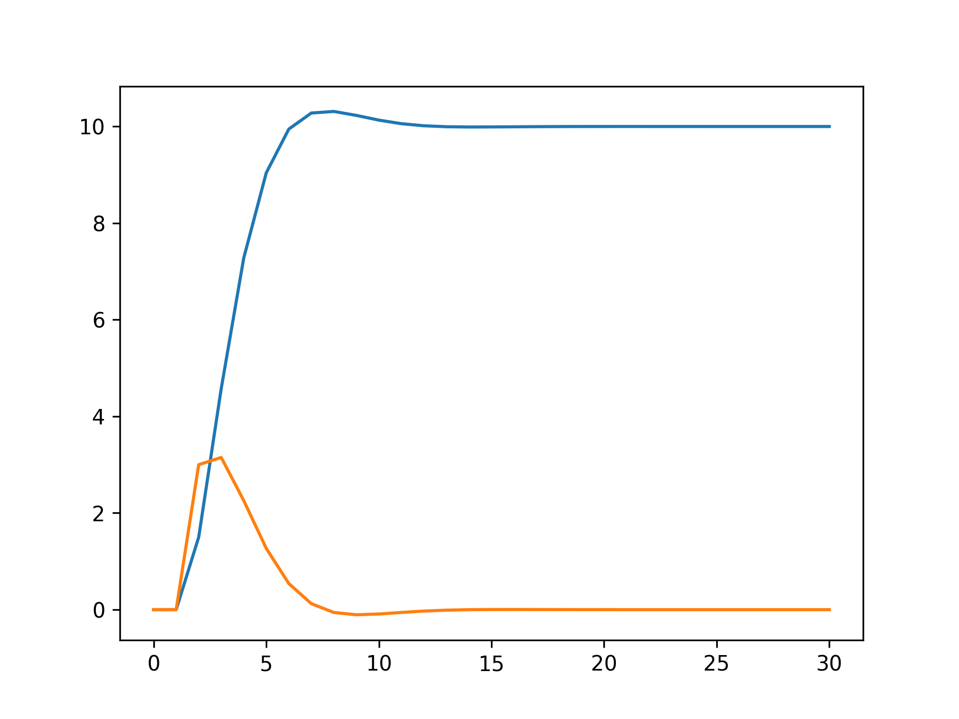
Notice that you can easily see the points in which the control loop is computed, which immediately change the velocity of the particle.

Conclusion

In this first tutorial, I showed how I use Julia to simulate systems that have continuous and discrete parts. The concept was introduced by a very simple problem in which the position of a particle must be controlled using a discrete control loop.

I hope you could understand well the concept and how easy it will be to extend it to much more complex simulations. If I was not very clear, please, let me know in the comments! I will use all your advice to improve this and my future tutorials!

In the following, you can find the source code of this tutorial.

using DiffEqBase
using OrdinaryDiffEq

###############################################################################
#                                  Variables
###############################################################################

# Global variable to store the acceleration.
# This solution was selected just for the sake of simplification. Don't use
# global variables!
a = 0.0

# Parameters.
r = 10.0   # Reference position.
k = 0.3    # Proportional gain.
d = 0.8    # Derivative gain.

# Configuration of the simulation.
tf     = 30.0             # Final simulation time.
tstops = collect(0:1:tf)  # Instants that the control loop will be computed.
u0     = [0.0; 0.0]       # Initial state.

###############################################################################
#                                  Functions
###############################################################################

# Dynamic equation.
function dyn_eq(du, u, p, t)
    du .= [0 1; 0 0]*u + [0;1]*a
end

# CALLBACK: Control loop.
# =======================

# Condition function.
function condition_control_loop(u, t, integrator)
    return t in tstops
end

# Affect function.
function affect_control_loop!(integrator)
    global a

    p = integrator.u[1]
    v = integrator.u[2]

    a = k*(r-p) + d*(0.0-v)
end

cb = DiscreteCallback(condition_control_loop, affect_control_loop!)

###############################################################################
#                                    Solver
###############################################################################

prob = ODEProblem(dyn_eq, u0, (0.0, tf))
sol  = solve(prob, Tsit5(), callback = cb, tstops=tstops)